Open Purchase Orders

You get easily overwhelmed on a visit to Mike Bostok’s gallery. Visualisation is after all programmers most powerful shock-and-awe toolkit, and Bostok’s d3 has it in abundance!

After a bit of tinkering I settled on a new page for the Gallery with a combination of a line graph and scatter plot of open purchase orders.

As the Address Book Inquiry, the page is build with KnockoutJS and Bootstrap 4, using an AIS Aggregate Query to fetch the data and d3 to chart it.

AIS Aggregate Query

An aggregate functionality has been sitting in the API layer for some time and it’s really with AIS that it get’s a chance to shine.

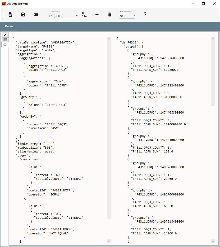
The aisDataBrowser is a handy tool for generating the request. For the open-pos page we want to sum up the open amounts and count order lines at status 400, grouped by requested date.

f4311 [count(f4311.drqj) group(f4311.drqj) sum(f4311.aopn) asc(f4311.drqj)]
all(f4311.nxtr=400 f4311.uopn<>0)

After successful submit, the request and result can be exported in json format.

The app.ts file has a bit of logic to read the result data from a file instead of requesting it from the AIS Server.

if (false) { // use demo data
    const response = require('../docs/sample.json');
    let total = 0;
    const rows = response.ds_F4311.output.map((r: any) => {
        total += Math.round(r['F4311.AOPN_SUM']/100)/1000;
        return {
            count: r.COUNT,
            total,
            date: r.groupBy['F4311.DRQJ']
        };
    });
    state.rows = rows;
    state.timeStamp = Date.now();
}

This is very convenient when finalising the output. Instead of having to request the data from the AIS Server after every tweak, just store the sample in a .json file and require it. This can also be useful for testing, just use different .json file for each test case. And finally, this allows a developer to work without access to an AIS Server, the only requirement is to understand the data structure – no working knowledge of Oracle E1 required.

D3 Charting

The key to understanding D3 is that you’re not drawing a linear graph or a scatter plot, but defining a series of objects that combined make up a linear graph or scatter plot.

The basic objects is the coordinates, or scales.

        // Scales
        this.x = d3.scaleTime()
            .domain(d3.extent(data, d => d.date))
            .range([0, this.width]);
        this.yTotal = d3.scaleLinear()
            .domain([0, d3.max(data, d => d.total)])
            .range([this.height, 0]);
        this.yCount = d3.scaleLinear()
            .domain([0, d3.max(data, d => d.count)])
            .range([this.height, 0]);

We have a date range on our x-scale and two y-scales, for totals and count.

Then we have a line for the total on the the x/y-total scale.

        // Define the line
        this.line = d3.line<IRow>()
            .defined(d => !isNaN(d.total))
            .x(d => this.x(d.date))
            .y(d => this.yTotal(d.total))
            .curve(d3.curveStepAfter);

        // Add the line
        this.svg.append('path')
            .attr('class', 'line')
            .attr('d', this.line(data));

And a scatter plot for the count on the x/y-count scale.

        // Add the scatter plot
        this.svg.selectAll('.dot')
            .data(data)
            .enter().append('circle')
            .attr('class', 'dot')
            .attr('r', 3.5)
            .attr('cx', d => this.x(d.date))
            .attr('cy', d => this.yCount(d.count));

And finally we add the three axis.

        // Add the axis
        this.svg.append('g')
            .attr('class', 'x axis')
            .attr('transform', `translate(0,${this.height})`)
            .call(d3.axisBottom(this.x));
        this.svg.append('g')
            .attr('class', 'y total axis')
            .attr('transform', `translate(${this.width},0)`)
            .call(d3.axisRight(this.yTotal));
        this.svg.append('g')
            .attr('class', 'y count axis')
            .call(d3.axisLeft(this.yCount));

There is a bit of additional logic to re-draw the chart with new data in the redraw function. Alternatively the chart could have been cleared and re-created with the same logic, but the transition logic in the redraw function is a far superior.

It takes a bit to get your head around D3 but when the mist start to lift, it makes such a perfect sense that it couldn’t be any simpler. And as can be seen in Bostok’s gallery and others, the results can be mesmerising!

- Title Picture -

In the absence of a shock-and-awe graph, I’m instead showing-off a picture of Kverkfjoll in Iceland. The rather innocently looking stream running from underneath the glacier was, until very recently, warm enough for a pleasant bath but has cooled to lukewarm – hopefully indicating that the volcano it originates from is resting peacefully for now.